Statistical data can be " distributed" (spread, dispersed, scattered) in a variety of ways.
See Shapes of Distributions.
 Bell-shaped Curve: |
There are certain sets of data where the data, when graphed, are symmetrical with a single central peak at the mean (average) of the data. The shape of the curve is described as bell-shaped with the graph falling off evenly on either side of the mean. Fifty percent of the distribution lies to the left of the mean and fifty percent lies to the right of the mean. Such graphs are called normal curves, and referred to as a normal distribution. The mean, median and mode are all the same in a normal distribution.
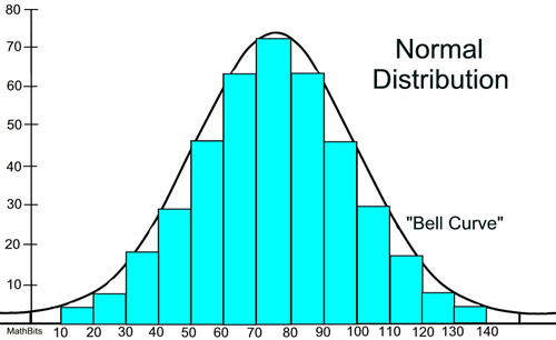
Notice how the histogram closely follows the form of the bell curve.
A normal distribution is the most widely known and used of all distributions. It is an extremely important statistical data distribution pattern occurring in many natural phenomena, such a blood pressure, machined parts, human height, error in measurement, IQ scores, sizes of snowflakes, lifespans of light bulbs, weights of loaves of bread, test scores, milk production in cows, etc. When data pertaining to these phenomena are graphed as histograms with data on the horizontal axis and the amount of data on the vertical axis, a bell-shaped curve (normal curve) may be created.
A normal distribution is actually a "family of distributions", since the mean and standard deviation, which determine the shape of the distribution, may differ from graph to graph.
Normal Distribution Basic Properties:
1. symmetric about the mean
2. the mean = the mode = the median
3. the mean divides the data in half
4. defined by mean and standard deviation
5. the curve is unimodal (one peak)
6. the curve approaches, but never touches, the x-axis, as it extends farther and farther away from the mean.
7. total area under the curve = 1.
(Characteristics of perfectly normal distributions.)
|
|
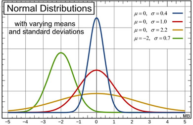 |
While the four normal curves shown above (at the right) share all of these basic properties, they are still unique
(different from one another) as to mean and standard deviation. |

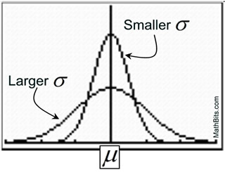
A normal distribution can have any mean and any positive standard deviation. The mean determines the line of symmetry of the graph, and the standard deviation determines how much the data are spread out.
The smaller the standard deviation, the more concentrated the data and narrower the graph. The larger the standard deviation, the more dispersed the data, and wider the graph.
|
 |
Population standard deviation = σ (small case Greek sigma);
population mean = μ (small case Greek mu). |
A Closer Look at the Shape of the Normal Curve: |
|
|
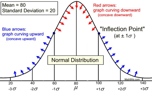
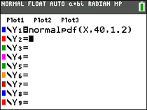
The graph shown above states that for this normal distribution the mean is 80 and the standard deviation is 20. The graph also shows that the mean (80) + 1 standard deviation (20) equals 100, the mean (80) + 2 standard deviations (40) = 120, and so on, to both the left and right sides of the mean.
Could you approximate the mean and standard deviation of a normal curve if this specific information was not stated on the graph? |
If you were given a normal curve, without being told the mean and the standard deviation, you could approximate this information based upon the shape of the curve.
• The mean in a normal curve divides the curve symmetrically. Therefore, the mean will pass through the highest point on the graph. In this example, it is logical to assume that the mean is 80.
• In a normal curve, the point at which the graph changes from curving downward to curving upward is called an inflection point and occurs at plus (or minus) one standard deviation from the mean. Examining a normal curve for this location will yield an approximation of the value of the standard deviation. In this example, an inflection point can be seen to be occurring around 100, or approximately 20 points above the mean. The standard deviation could be approximated to be 20.
(Think of an inflection point as the center point when drawing a figure eight. It is the point where the bending changes from the top of the 8 to the bottom.) |
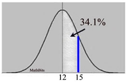
| Percentages Under a Normal Curve: |
As seen in the previous section, the standard deviation can be used to sub-divide the space (the area) under a normal curve, starting from the mean. Each of these sub-divided sections can be used to represent a portion (a percentage) of the data falling into these sections of the graph. The normal curve actually shows how likely it is to find a value within a specific distance from the mean.
Using 1 standard deviation to create the subdivisions: |
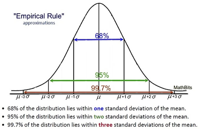
The most popular subdivision utilizes distances from the mean in increments of one standard deviation of that specific normal curve.
When dealing with a normal curve:
• approximately 68% of the data will fall within one standard deviation of the mean
(between the mean minus one standard deviation and the mean plus one standard deviation),
•
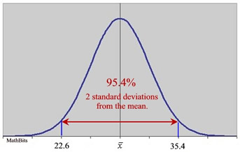
approximately 95% of the data will fall within two standard deviations of the mean
(between the mean minus two standard deviations and the mean plus two standard deviations),and
• approximately 99.7% of the data will fall within three standard deviations of the mean
(between the mean minus three standard deviations and the mean plus three standard deviations).
These three facts make up what is referred to as the Empirical Rule (or the 68-95-99.7 Rule).
 |
These percentages represent the probability of data falling within given distances from the mean of a normal curve. The probability of the data falling somewhere on the graph is 100%. Expressed as decimals, we have 0.68, 0.95, 0.997, and 1.0. There is a correspondence between probability and area under the curve that will be discussed in Understanding Z-Scores. |
|
NOTE: Normal distributions may also be referred to as normal probability distributions.
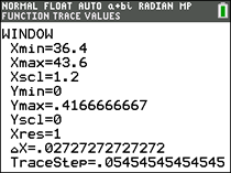
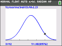
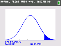
Using ½ of 1 standard deviation to create the subdivisions: |
It is possible to subdivide the area under a normal curve into smaller intervals, such as widths of 0.5 standard deviations, as shown in the graph below. The addition of the percentages in this graph will be slightly different from the Empirical Rule values which are rounded approximations. These smaller subdivisions would be used when information presented in a question falls on the increments of one-half of one standard deviation from the mean.
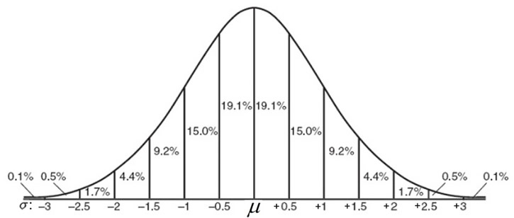
Graph based upon 0.5 standard deviation subdivisions.
[68.2% - 95.4% - 99.8%]
 Not all data is normally distributed. Not all data is normally distributed. |
Statisticians use both simple and complex mathematical techniques to determine if a data set is distributed normally. The more data that is available, the more likely it can be determined if the population data is normal or not.
The simplest test for normality is to make a histogram of the data. If the shape of the distribution resembles a bell curve, the data is likely normal. Further examinations such as whether the mean equals the median, and whether approximately 68% of the data is within one standard deviation of the mean, 95% within two standard deviations and 99.7% within three standard deviations may help verify if the data comes from a population that is normally distributed.
Example:
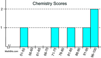
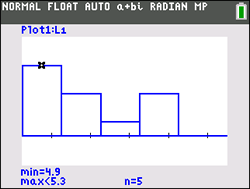
Kayla's scores in Chemistry this semester were rather inconsistent: 100, 85, 55, 95, 75, 100. What percent of Kayla's scores are within one standard deviation of the mean?
|
|
Solution: At first reading, you may want to jump to the conclusion that the answer is 68%, because the Empirical Rule tells us that 68% of the data falls within one standard deviation of the mean (for a normal distribution). But this is NOT a normal distribution.
|
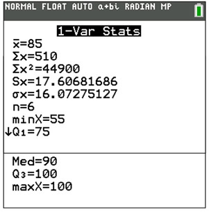
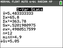
Looking at the histogram above, it can be seen that this data will not resemble a bell-shaped curve. With a little mathematical computation, (or a little help from the graphing calculator) it can be shown that the mean and the median are not equal.
• The mean for this set: 85
• The population standard deviation: 16.07275127
• The interval for one standard deviation about the mean: from 85 - 16 to 85 + 16
or (69 to 101)
• The number of scores in this interval: 5
• The total number of scores: 6
• Percentage: 83.33333333% |
This is an extremely small data set. In this question, the data is the "population" since we are only looking at Kayla's scores (not in relation to a bigger set of school-wide scores).
If Kayla's scores were part of a bigger set of school-wide scores, this data would not necessarily tell us that the larger "population" was also not normally distributed. This would be too small of a sample set to be used to make inferences about the larger population. |
|
If a small sample set appears to be normal, it is dangerous to make the assumption that the population is also normal. Such an assumption may lead to an incorrect statistical analysis, and incorrect implications regarding the data.
More sophisticated tests for normality require computer software packages and complex calculations.
|